Tutorial
Table of contents
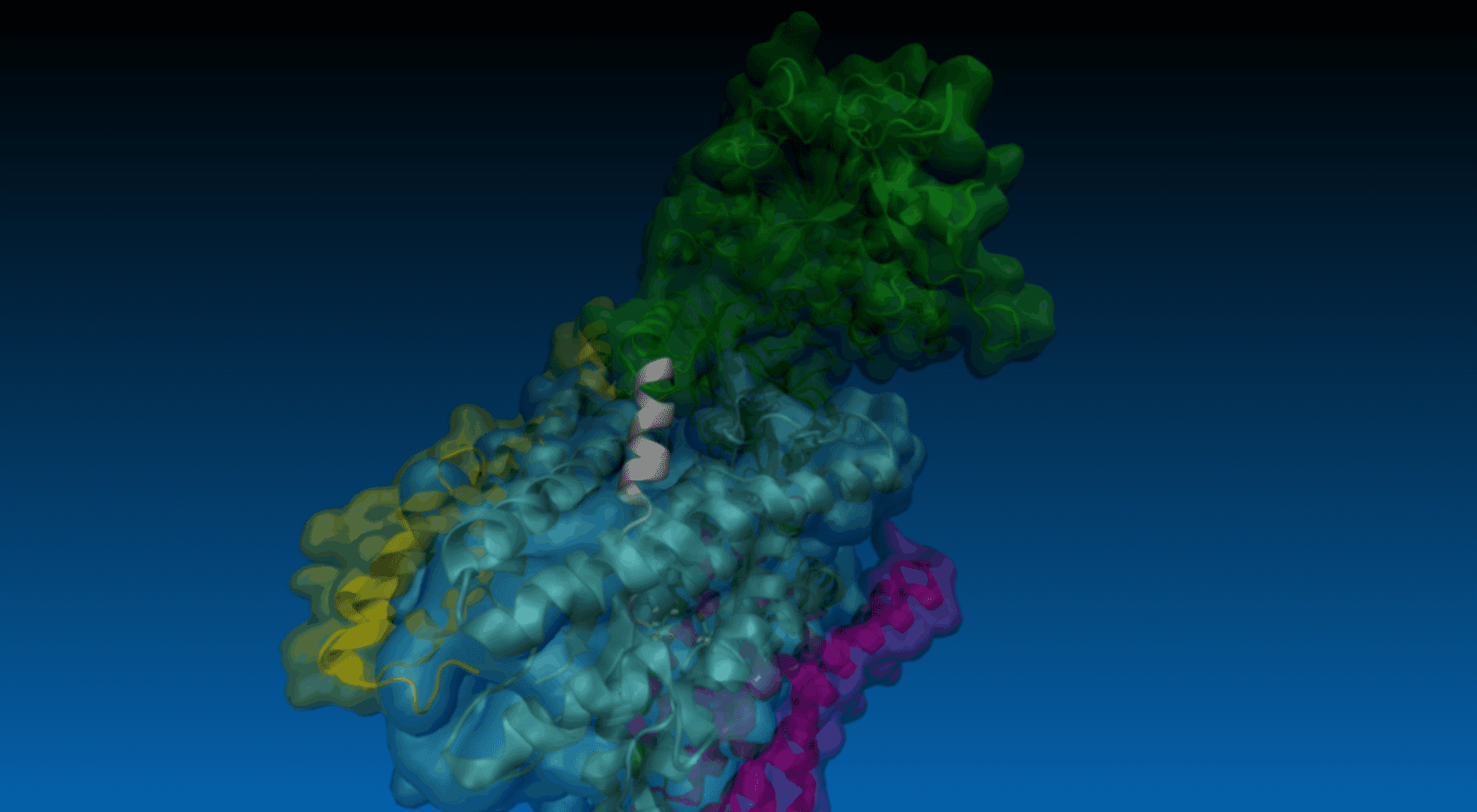
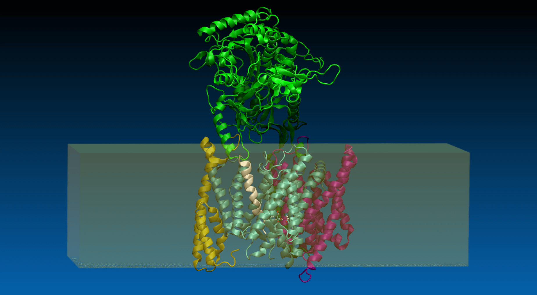
SMD (steered molecular dynamics) – method description
Steered molecular dynamics is a non-equilibrium molecular dynamics method ideal for studying the resistance encountered by a molecule when it is moved in a certain direction. The resistance experienced by the molecule is expressed as a force required to overcome it. Speaking more precisely, a virtual atom moving with a constant velocity (the velocity value and its vector are specified by the user) is connected to the real atom (ie. SMD atom)* of the studied molecule by a virtual spring (spring force constant value and the SMD atom are also specified by the user). The force is applied to the virtual atom, its value adjusted automatically in order to maintain the constant velocity of the virtual atom. The force value and the coordinates of SMD atom are monitored and recorded throughout the simulation. The data recorded during a SMD simulation allow for calculation of the energy barriers encountered by the molecule during its journey ( ). By sampling different pulling directions it is possible to explore the degrees of freedom of a molecule in a studied system as well as to obtain the reaction coordinates that can be used for umbrella sampling (another sampling method useful for mapping the energy landscape of a studied system).

* In GS-SMD the Cα atom of the C-terminal residue of the substrate is defined as an SMD atom.
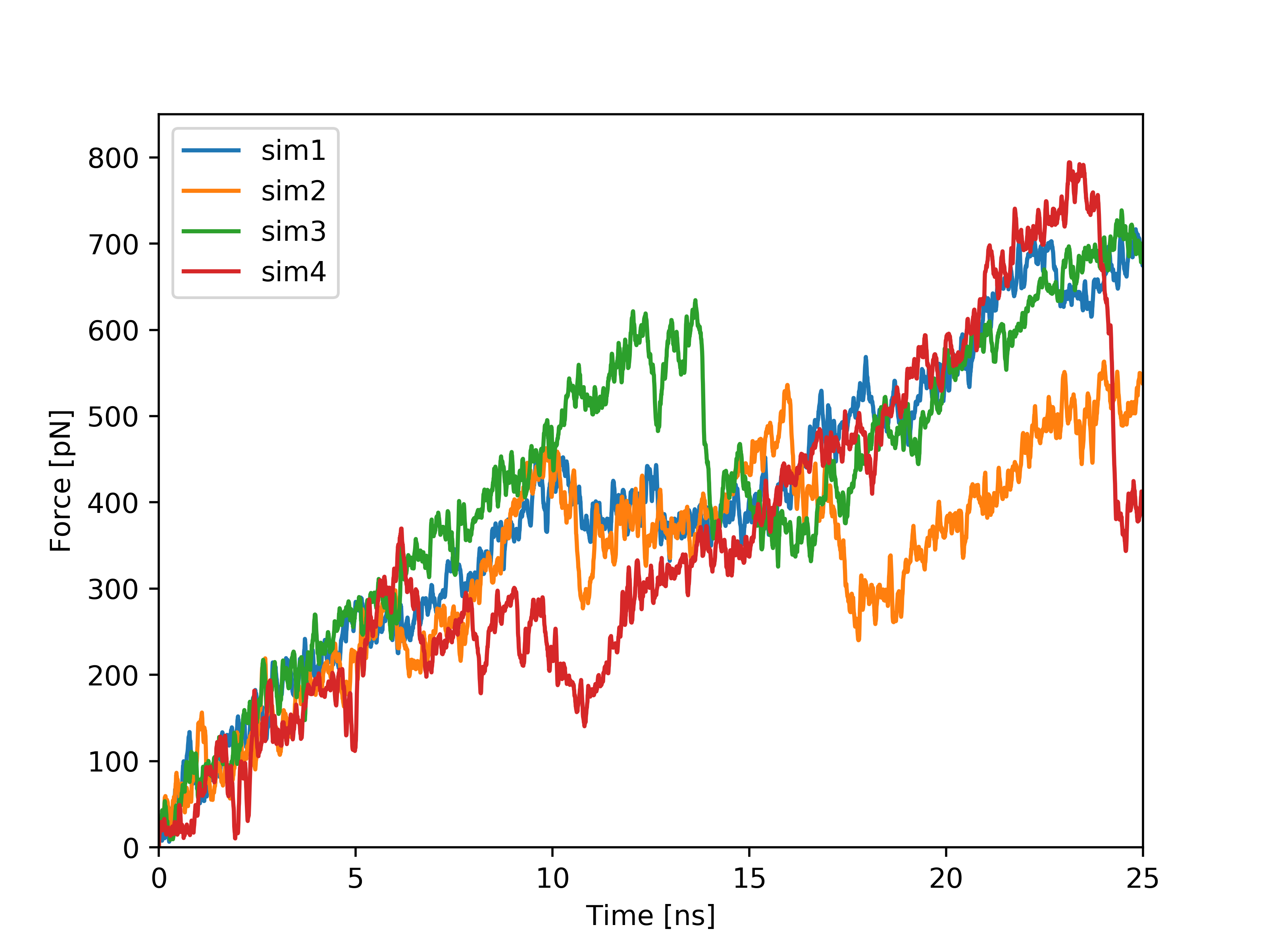
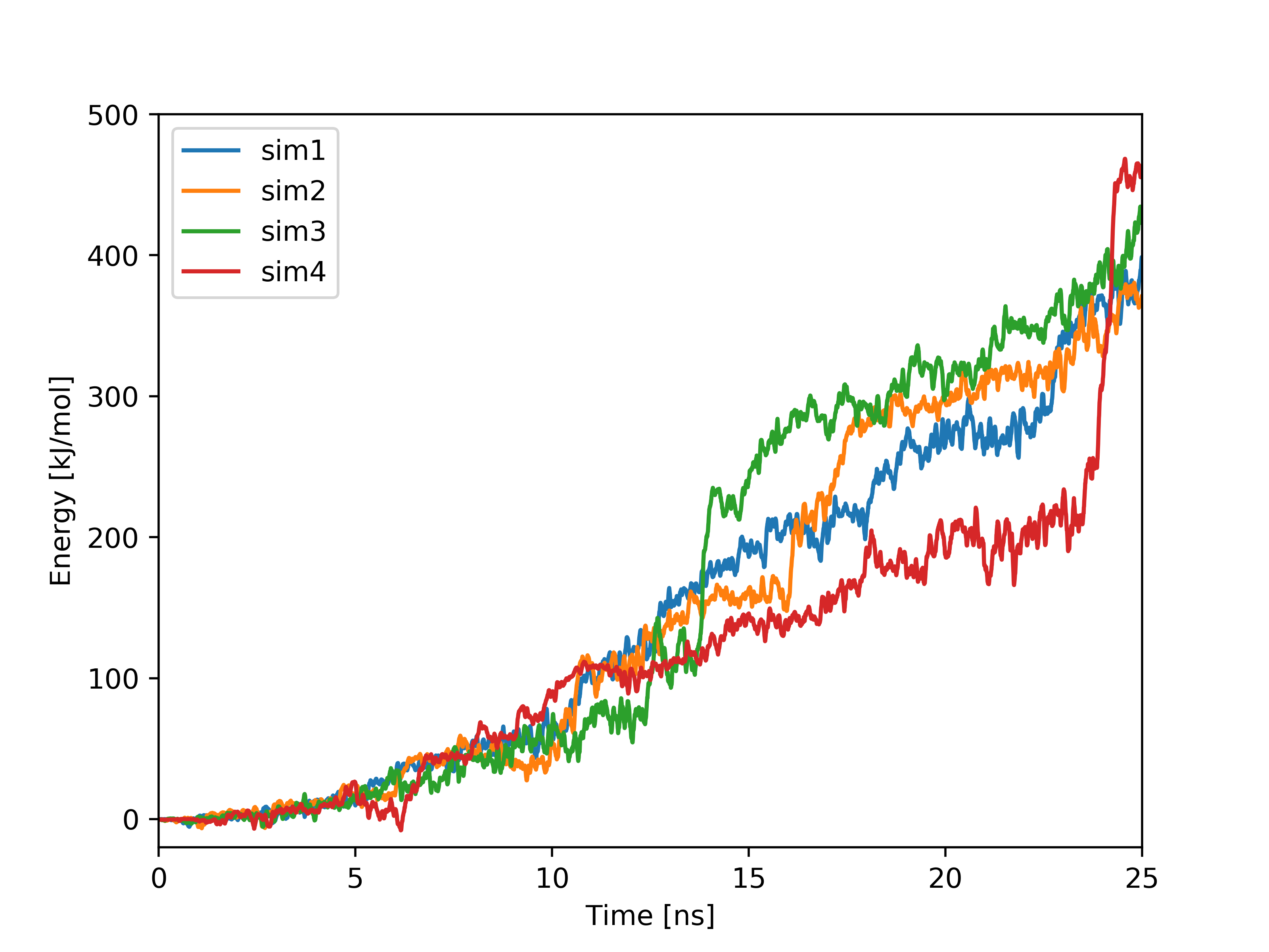
Plots based on SMD simulations showing force and work/energy vs. time. Results from four simulations with identical SMD parameters of the same system GS-APP (γ-secretase-amyloid precursor protein) are shown on each figure.
Example of analysis of single SMD trajectory (trajectory in red in F/t plot)
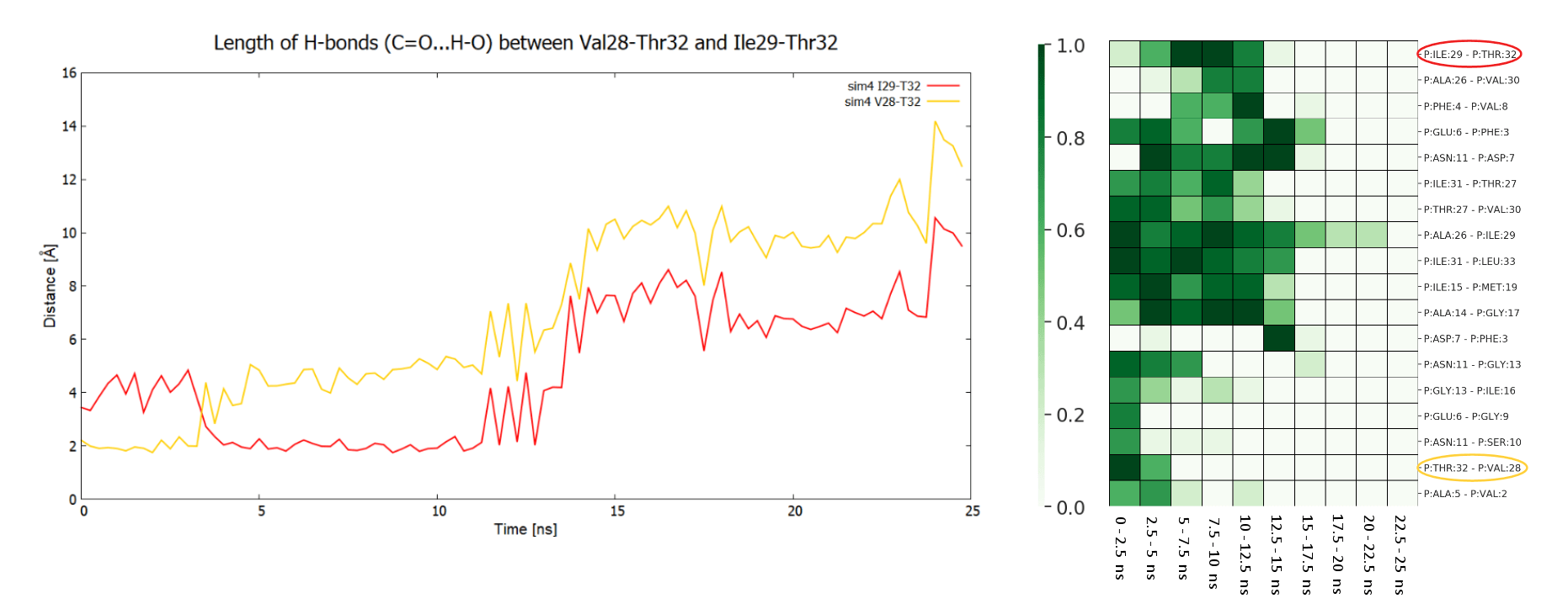
By analyzing the trajectory the user can identify the hydrogen bonds that are creating/breaking during the simulation. The linear plots show distances between the interacting atoms from two selected residues at C-terminus of APP (1-33) substrate (Val28-Thr32 in orange, and Ile29-Thr32 in red). The plots indicate presence of hydrogen bond between side chain of Thr32 and carbonyl group of Val28 and then Ile29, That bond hopped from residue 28 to 29 at 3 ns, and was broken at about 14 ns - that event is associated with significant force drop in F/t plot. The same events can be seen in HeatMap (the interactions in the above residue pairs are encircled) together with other hydrogen bond creating/breaking events between other residues. The presented HeatMap shows frequencies [0-1] of hydrogen bonds within APP substrate for different time intervals. Since such analysis is highly dependent on GS-substrate/mutant pair, it is not part of the server and should be done on individual basis.
In order to submit your own input for a simulation press the button or click the “MD&mut” label at the top action bar.
A “Molecular dynamics & mutations” window pops out.
Timeline
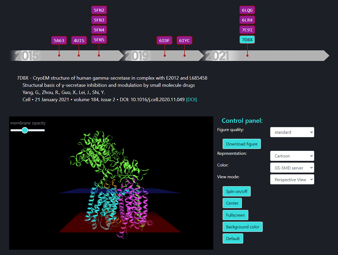
In this page the structures of γ-secretase complex deposited in Protein Data Bank (PDB) can be seen. All structures deposited so far are available on a timeline. By selecting the PDB ID the structure of γ-secretase shows up in a window and one can visualize its structure using options from the control panel. The details of citation with a DOI link are shown above the structure window.
Molecular dynamics & mutations
By clicking the button one can fill the whole ‘Molecular dynamics & mutations’ form with a sample input data.
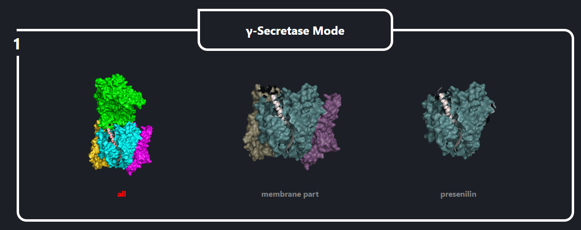
In the field number 1 labeled ‘γ Secretase Mode’, the user selects how large fragment of the γ-secretase complex should be included in the simulations (the appropriate protein fragment is highlighted when clicked)
- All – the whole γ-secretase complex: Nicastrin (chain A), residues 34-700; Presenilin-1 (chain B), residues 73-298, 374-467; Aph1-A (chain C), residues 2-244; PEN-2 (chain D), residues 2-101 are included in the simulation
- Membrane part – only transmembrane part of the γ-secretase complex: transmembrane helix of Nicastrin (chain A), residues 664-700; Presenilin-1 (chain B), residues 73-298, 374-467; Aph1-A (chain C), residues 2-244; PEN-2 (chain D), residues 2-101 are included
- Presenilin – only the catalytic subunit of γ-secretase, Presenilin-1 (chain B), residues 73-298, 374-467 is included (the long loop between transmembrane helices TM6 and TM7 is not determined)
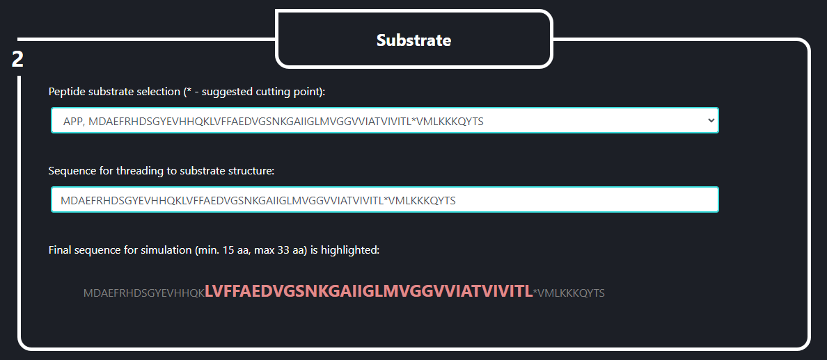
In the field no. 2 labeled ‘Substrate’ the user specifies what substrate is going to be used in the SMD simulation. In the upper line (‘Peptide substrate selection’) the initial version of substrate peptide (a template for sequence threading) is selected from a pop-up menu which appears when the line is clicked. In the lower line (‘Sequence for threading to substrate structure’) the sequence to be threaded is specified by the user. The cleavage point (marked by ‘*’) is used as a reference position for a sequence threading. The final sequence for the simulation is highlighted in red below the lower line. The final sequence should be between 15 and 33 AA long. This sequence will be threaded to the substrate structure in PDB ID:6IYC γ-secretase.
Here is the list of Selected substrates of γ-secretase with known cleavage point (available in Substrate input)
| Protein Name | UniProt ID | Membrane region sequence |
| Alcadein α (Calsyntenin-1) | O94985|CSTN1_HUMAN Q9EPL2|CSTN1_MOUSE | VVPSTAT*VVIVVCVSFLVFMIIL*GVFRIRAA |
| Alcadein β (Calsyntenin-3) | Q9BQT9|CSTN3_HUMAN | MIPSAATLII*VVCVGFLVLMVVLG*LVRIHSLH |
| Alcadein γ (Calsyntenin-2) | Q9H4D0|CSTN2_HUMAN | SVVPSIAT*VVIIISVCMLVFVVAM*GVYRVRIA |
| APLP1 | Q03157|APLP1_MOUSE P51693|APLP1_HUMAN | GVSREAVSGLLIMGAGG*GSLIVL*SMLLLRRKKP |
| APLP2 | Q06481|APLP2_HUMAN Q06335|APLP2_MOUSE | FSLSSSA*LIGL*LVIAVAIATVIVISL*VMLRKRQY |
| APP | P05067|A4_HUMAN | VGSNKGAIIGLMVGGVV*IATVIVITL*VMLKKKQY |
| CD44 | P16070|CD44_HUMAN | PQIPEWLIILASLLA*LALILAVCI*AVNSRRR |
| CSF-1R | P09581|CSF1R_MOUSE | SLFTPVVVACMSVMSLLVLLLL*LLLYKYKQK |
| E-Cadherin | Q90762|CADH6_CHICK P09803|CADH1_MOUSE P12830|CADH1_HUMAN P19022|CADH2_HUMAN P15116|CADH2_MOUSE P33151|CADH5_HUMAN | LQIPAILGILGGILALLILILLLLLFL*RRRRA |
| EpCAM | P16422|EPCAM_HUMAN | MQGLKAGVIAVIV*VVVIAVVAGIV*VLVISRKKR |
| EphB2 | P54763|EPHB2_MOUSE | EKLPLIVGSSAAGLVFLIAVVVI*AIVCNRRG |
| GHR | P16882|GHR_MOUSE P19941|GHR_RABIT | EEDFRFPWFLIIIFGIFGLTVMLFV*FIFSKQQRI |
| IL-1R2 | P27930|IL1R2_HUMAN | TTVKEASSTFSWGIV*LAPLS*LAFLVLGGIWMHRRCK |
| Neuregulin-1 | Q6DR98|Q6DR98_MOUSE | LYQKRVLTITGICIAL*LVVGIMC*VVAYCKTKKQ |
| Notch-1 | Q01705|NOTC1_MOUSE | PAQLHFMYVAA*AAFVLLFFVGCG*VLLSRKRR |
| Notch-2 | O35516|NOTC2_MOUSE | PERTQLLYLLAVAVV*IILFIILLG*VIMAKRKRK |
| Notch-3 | Q61982|NOTC3_MOUSE | PSVPLLPLLVA*GAVLLLVILVLG*VMVARRKRE |
| Notch-4 | P31695|NOTC4_MOUSE | ANQLPWPVLCSPVAG*VILLALGALL*VLQLIRR |
| p75 NTR | P08138|TNR16_HUMAN | GTTDNLIPVYCSILAAVV*VGLVAYIAFKRWNS |
| Podoplanin (PDPN) | Q86YL7|PDPN_HUMAN | STVTLVGIIVGVLLAIGFIGAIIV*VVMRKMS |
| PTK7 | Q13308|PTK7_HUMAN | KMIQTIGLSVGAAVAYIIAVLG*LMFYCKKRC |
| Syndecan-3 | O75056|SDC3_HUMAN Q64519|SDC3_MOUSE | ERKEVLVAVIVGGVVGALFAAL*VTLLIYRMKK |
| VEGFR-1 (FLT1) | F1MDD9|F1MDD9_BOVIN | KSNLELITLTCT*CVAATLFWLLL*TLFIRKMKR |
The ‘*’ sign indicates the experimentally identified cleavage position/s in all sequences.
For other substrates available to select in the GS-SMD server, the cleavage sites are unknown. Therefore, the ‘*’ sign is placed before last but 2 position of the transmembrane sequence, which is the most common cleavage site among the substrates described above. Such positioning is just indicative and should be considered by the user according to his/her knowledge. A complete list of all substrates can be found in a recent publication https://doi.org/10.1016/j.semcdb.2020.05.019
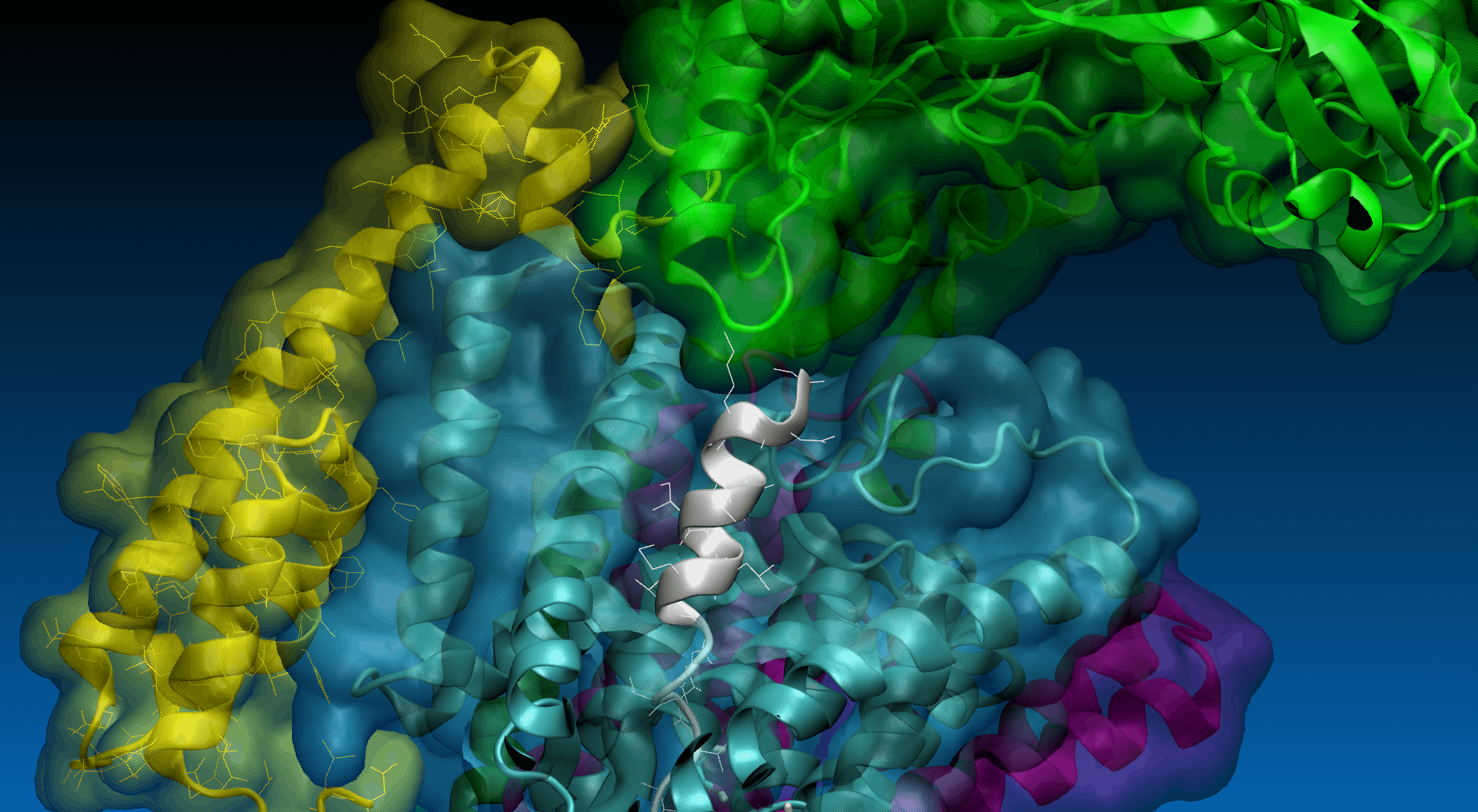
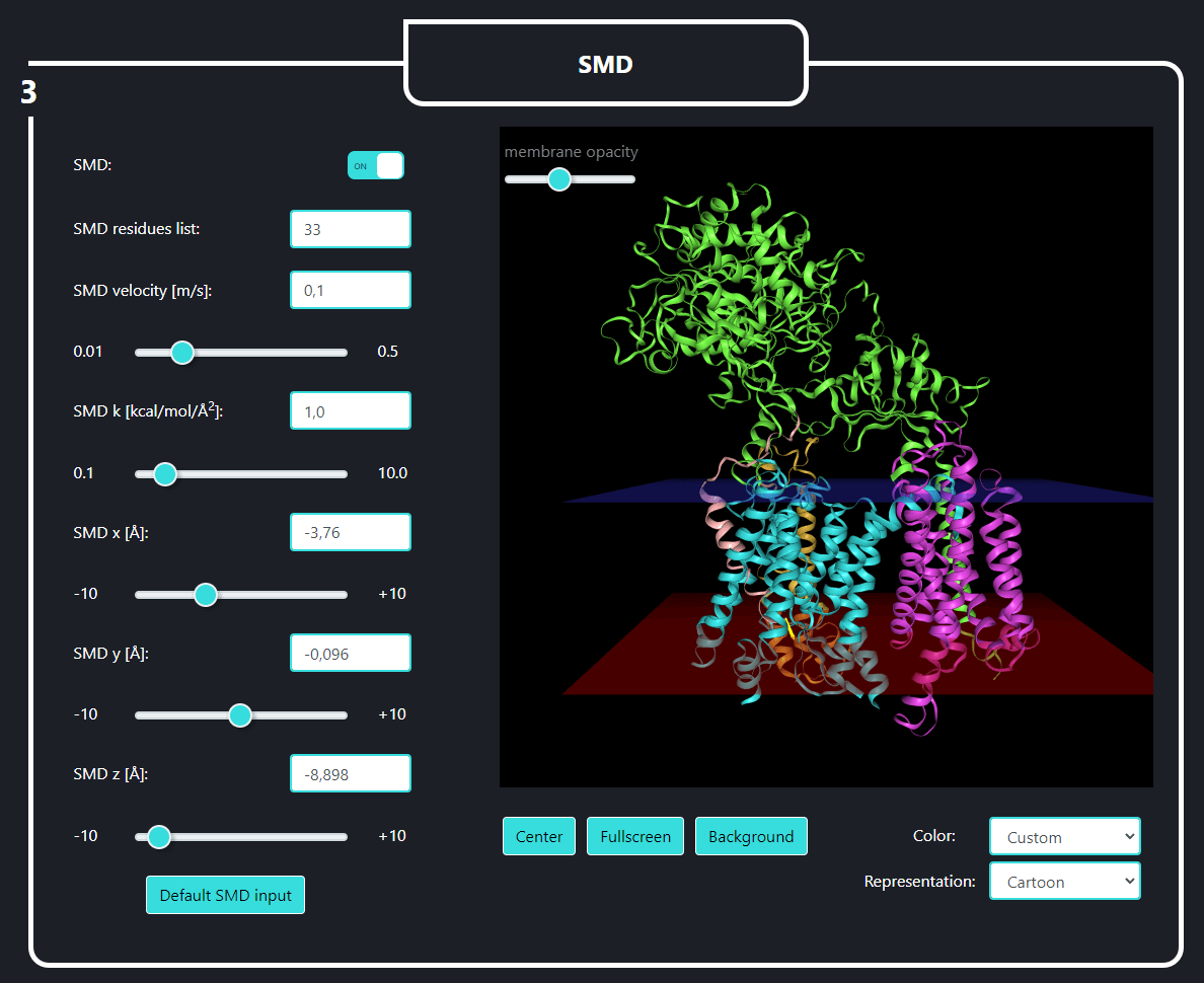
In the field no. 3 labeled ‘SMD’, the user provides the parameters for SMD simulation, namely: SMD velocity [m/s], virtual spring force constant [kcal/mol/Å2] and coordinates of the force vector [Å]. One can pull not only the last residue (No. 33, default) of the substrate but also any set of substrate residues (chain E) by specifying them in the 'SMD residues list' field.
Magnification of the structure showing the pulling direction selected by user (yellow arrow).
- sets all the SMD parameters to their default values
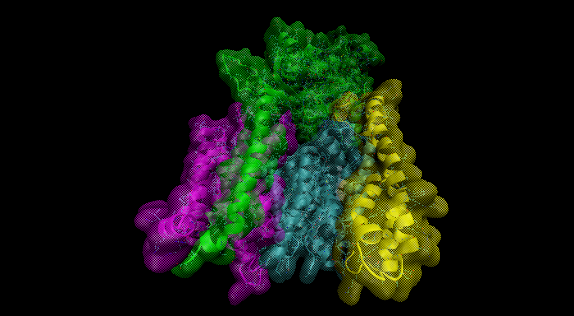
To the right is the visualization of gamma-secretase with a substrate. The membrane opacity can be adjusted using the slider above. The user can navigate the visualization state with the four buttons below:
- centers the whole complex
- toggles the full screen view (press ‘esc’ to exit the full screen mode)
- changes the background color from black to white or from white to black
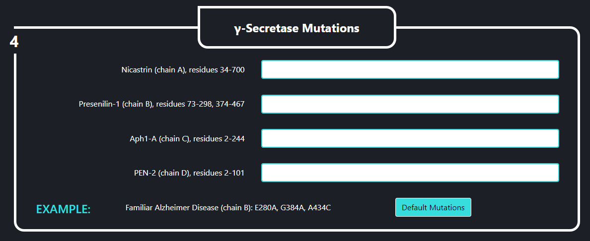
In the field no. 4 labeled ‘γ-Secretase Mutations’ the user can introduce specific mutations into the γ-secretase complex, that will going to be used in the simulation. Each line stands for a different subunit of the enzyme. Mutations should be specified using one letter code and a following format: ANB where “A” is the residue to be mutated, “N” is the residue number and “B” is a destination residue. For instance, if you want to mutate histidine 100 to alanine you should type “H100A”
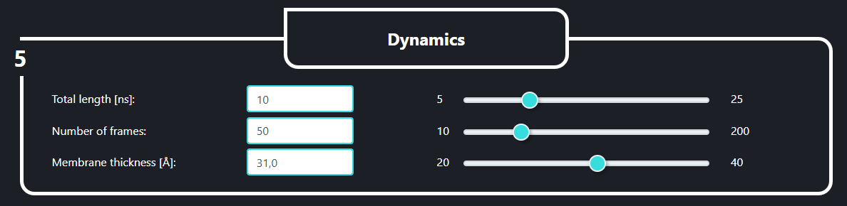
In the field no. 5 labeled ‘Dynamics’ the user can set the length of the simulation (Total length [ns], default value is 10), the number of frames in the trajectory (number of frames, default value is 100, please note that the more frames you decide to save the heavier the output files will be) and the implicit membrane thickness (Membrane thickness [Å], default value is 31.0).
After adjusting all the parameters click to start the SMD simulation.
If you wish to set all the parameters to their default values, click
Examples
In order to see some sample results you should click ‘Example1’ and ‘Example2’ at the top menu.
Example 1: pulling of C-terminus (Cα atom of residue 33) of APP in all γ-secretase structure.
Example 2: pulling of N-terminus (residues 1-21) of APP in PS-1 structure. An arrow indicates pulling of center of mass of selected residues (Cα atoms).
Example 3: comparison of four SMD trajectories (pulling of APP) using the Interaction frequency analysis.
Analysis of single MD
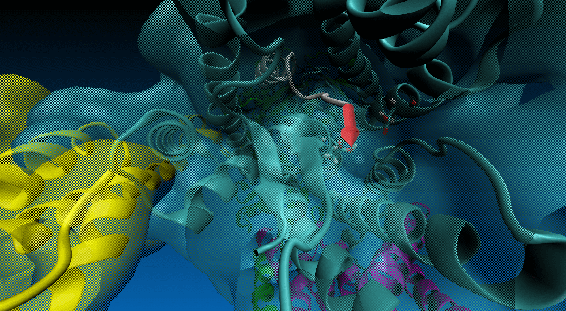
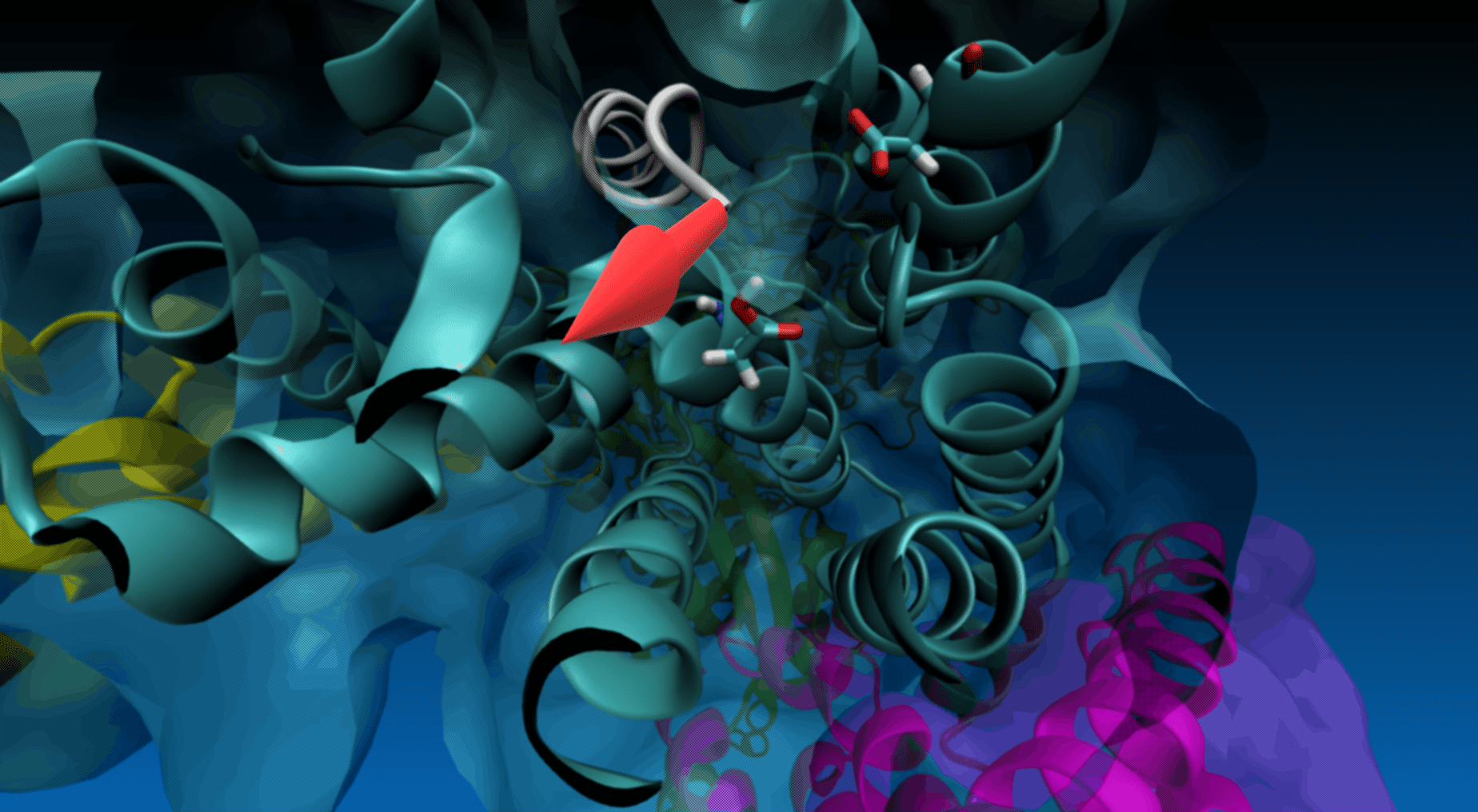
Magnification of the structure showing the pulling direction (yellow arrow) and the distance of the virtual atom to SMD atom (in red).
Downloads
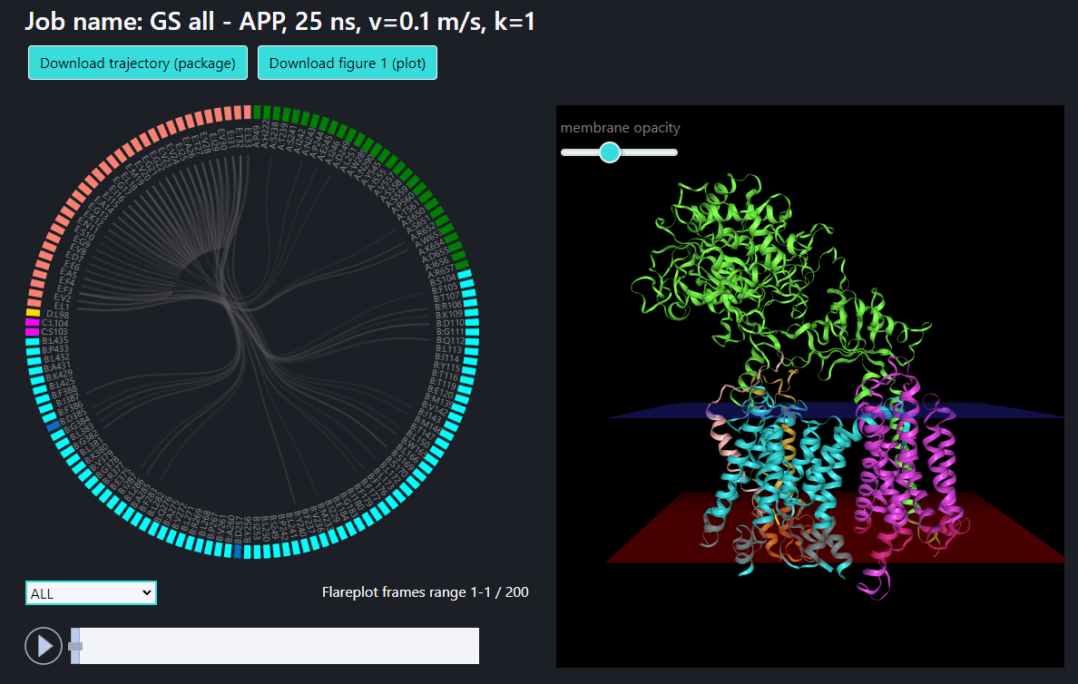
Download the trajectory package as zip file containing trajectory (in DCD format) and the files for making flare plots and frequency analyses (button: above the flare plot)
Download the current view of the flare plot (button above the flare plot)
Download the current view of the structure visualization (button below the trajectory visualization window)
Flareplot control
Interaction type selection – below the flareplot there is pop-up-on-click-menu where the user can select the interaction types to be visualized (such as: salt bridges, hydrogen bonds, aromatic, VdW or all types at once). The interactions of the substrate to the subunits of γ-secretase, as well as internal interactions in the substrate are displayed.
Slider (frame/frame range) selection – using the slider below the flareplot window the user can select the frame for which the interactions should be visualized. In addition the slider is synchronized with a NGL visualization of the trajectory, therefore the user can simultaneously track the structural changes of the system and the changes in the interaction network. The slider allows for selection of a range of frames as well and in such case the interactions are shown for more than one frame (the line thickness is proportional to the frequency of the particular interaction within a selected range of frames) and the NGL visualization show the first frame from the selection.
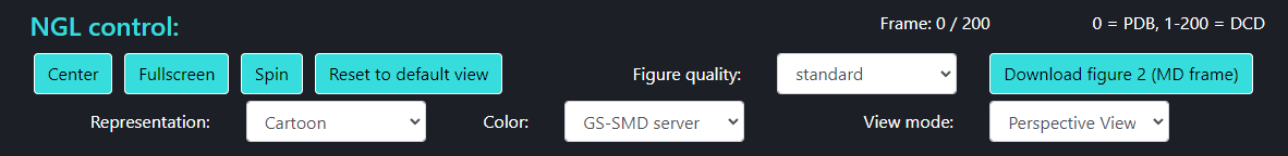
NGL control
- Membrane opacity - The slider on NGL window – allows to adjust the opacity of the membrane representation (blue and red surfaces representing the membrane borders)
- - centers the structure
- - activates the full screen view (to exit the full screen press ‘Esc’)
- - activate a slow rotation (spinning) of the system
- - restores default view settings
- Representation – a pop-up menu where the user can choose a representation of the structure (such as: cartoon, backbone, surface, etc.)
- Figure quality – a pop-up menu where the user can adjust the quality of the visualization (affects also the quality of the image saved when using described in ‘Downloads’ section)
- Color – a pop-up menu where the user can select the coloring scheme for the structure visualization. Available coloring methods are: GS-SMD server, which is coloring by protein chain; rainbow
- View mode - a pop-up menu allowing to switch between perspective and orthographic view
Charts
Below the flareplot and NGL visualization the plots of Force in a function of Time and of Energy/Work in a function of Time are shown. Both plots are based on SMD simulations results
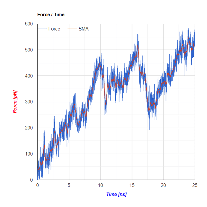
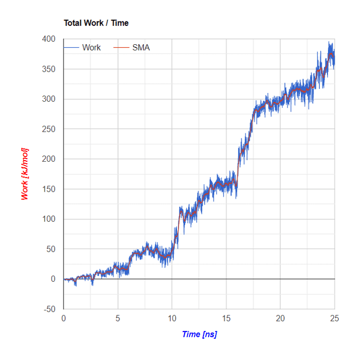
SMA - Simple Moving Average
Simple Moving Average (SMA) uses a sliding window to take the average over a set number of time periods. It is an equally weighted mean of the previous n data points.
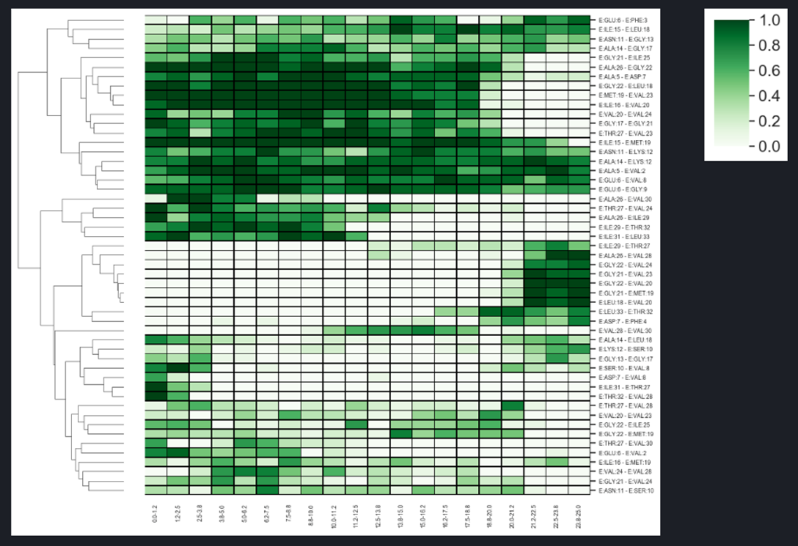
The heatmap showing changes in the network hydrogen bonds of the substrate during SMD simulation.
The trajectory is divided into several parts and the frequency analysis is applied.
Below is the Secondary structure plot together with Job information
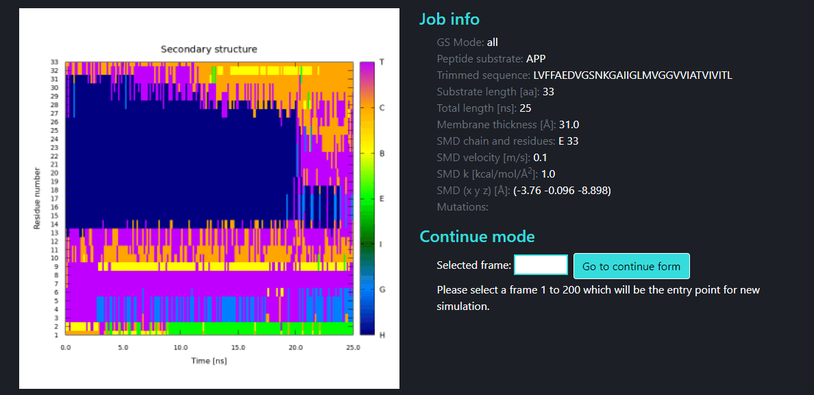
H - α-Helix, G - 310-Helix, I - π-Helix, E - Strand, B - Bridge, C - Coil, T - Turn.
Compare jobs
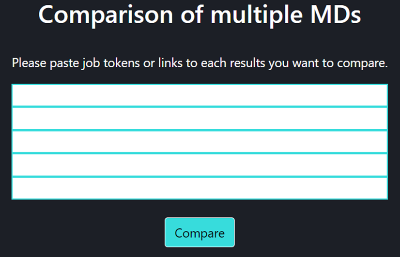
On this page one can add any number of trajectories (via their tokens) for their comparisons using Analysis of multiple MD page.
Analysis of multiple MDs
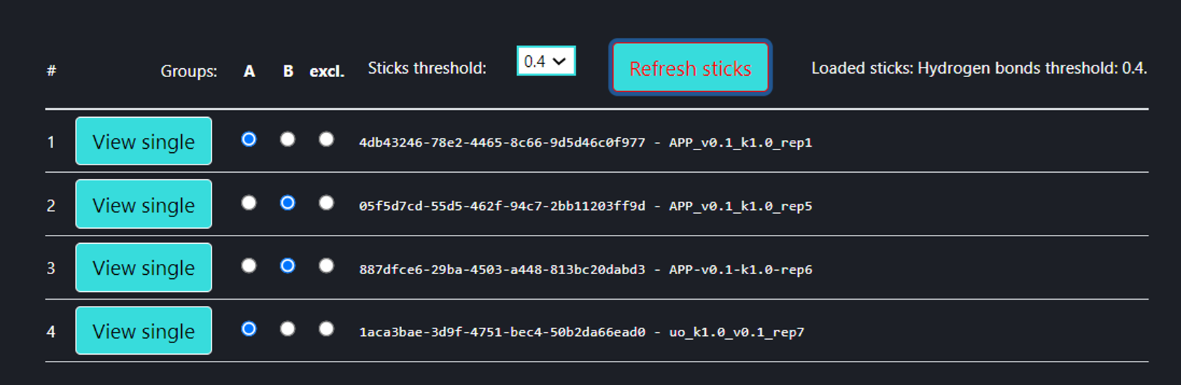
On this page the user can compare multiple MD trajectories (any number, the four above is only an example) which are introduced via “Compare jobs” page. In the trajectory selection menu (the figure above), the user can select multiple trajectories into groups A and B, to be compared with one another. By default, all trajectories are excluded from comparison (“excl.” field checked), and one can leave some trajectories excluded. If at least one trajectory has been selected for groups A and B, then pressing [Refresh sticks] button makes the analysis (Interaction frequency difference analysis) with the particular threshold. The user can review each of the trajectories in a ‘Single Trajectory’ mode by clicking [View single] button next to trajectory number.
Comparing only two trajectories may be not enough since many interaction frequency differences between two single trajectories can be random. The more trajectories each set contains, the more likely it is that the frequency difference of a certain interaction between the two sets is not random but is due to a change in the simulation conditions (different direction of pulling, spring constant, membrane thickness, GS mode, mutation*, etc.).
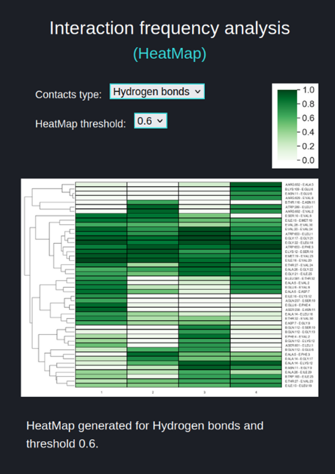
The HeatMap (figure above) visualizes the frequencies of residue-residue interactions (contacts) involving the substrate (chain E) calculated for each of the trajectories included in the comparison. The contact frequency values span between 0 and 1. Frequency 1.0 means that a certain interaction is observed in 100% of the trajectory frames, frequency 0.5 is observed in 50% of the trajectory frames, frequency 0 % means that this interaction was not found in particular trajectory but this interaction is collected because it exists in other selected trajectories and is above the threshold.
The user sets two parameters for the heatmap:
- 'Contacts type' (Hydrogen bonds (default), Salt Bridges, Aromatic) for which frequencies are to be compared between trajectories and visualized as a heatmap.
- 'HeatMap threshold' (default value 0.6) which narrows the number of interactions included in the HeatMap, displaying only those interactions for which the frequency range is equal or greater than ‘HeatMap threshold’ value.
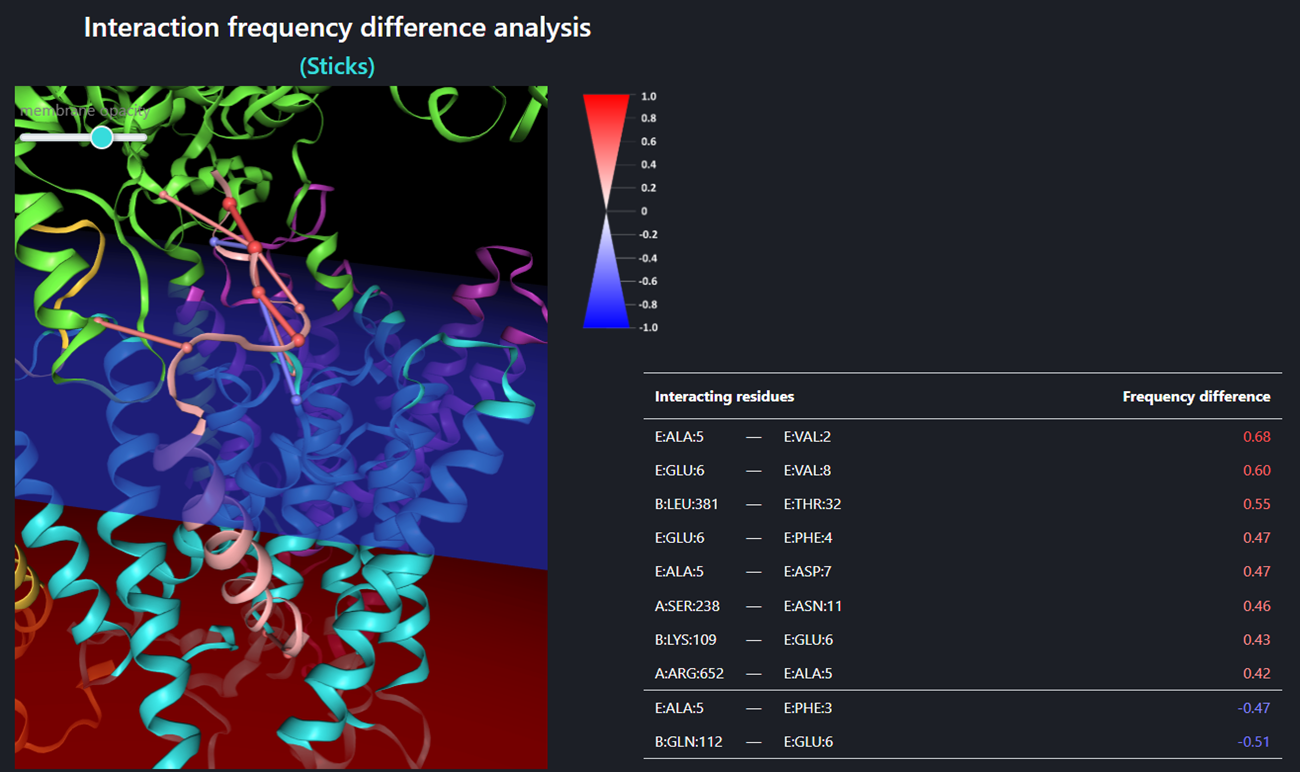
The Interaction frequency difference analysis (so called Sticks – the figure above), identifies only those interactions for which the frequency difference (between trajectory sets A and B) is equal or greater than the ‘sticks threshold’. The stick color represents the value of a frequency difference for that interaction between trajectory sets A and B (the legend for stick color is shown close to the window of the structure visualizer). Using buttons the user can customize the view of the structure – the menu is the same as for the single trajectory. Sticks threshold (its default value is 0.4) represents a minimal difference between frequencies of a certain interaction in sets A and B required to show that interaction as a stick and include the frequency difference of that interaction in the table below. The lower the threshold the more interactions will be included. In order to display/refresh sticks please click the [Refresh sticks] button.
The specific values of the frequency differences are listed in the table below the visualizer menu. Interactions are sorted by their frequency difference. The same coloring method is applied for frequency differences as for graphical sticks: positive frequency differences (meaning that the a certain interaction was recorded more often in set A than in B) are shown in red while negative frequency differences (meaning that the a certain interaction was recorded more often in set B than in A) are shown in blue. The higher the absolute value of the frequency difference is, the more intense the color.
* The algorithm identifies residues not only by their numbers but also by their names. Therefore, the same interaction formed by a mutated and un-mutated residue will be interpreted as two distinct interactions, yielding two separate lines in the heatmap and two separate sticks.
SMD-off optimization
(recommended to use after SMD simulation)
During SMD pulling, the applied force enables observation of the process of substrate unwinding and relocting towards an intracellular site. However, the usage of such restraints generates some non-biological frictions that can slightly deform the temporary substrate confomation in the active site. Due to that, we provide the SMD-off option and recommend to use it after the SMD simulation, for short optimization of a chosen complex conformation. The frame of concern can be picked from SMD trajectory by using „Continue mode” option, available in results page. The SMD-off option is placed in „SMD” field in the job parameters form.
For the SMD simulations presented at the top of the tutorial (with APP substrate) the example conformation with the shortest distance (it was about 5 Å on average) between catalytic residue D257 and substrate V30 (a cleavage site) was selected for SMD-off optimization. A violin plot below shows the distances between the sidechain oxygen atom of D257 and the main chain oxygen atom of V30. Presence of the values below 4 Å indicates a possibility of the catalytic cleavage event, as a water molecule mediates the reaction.
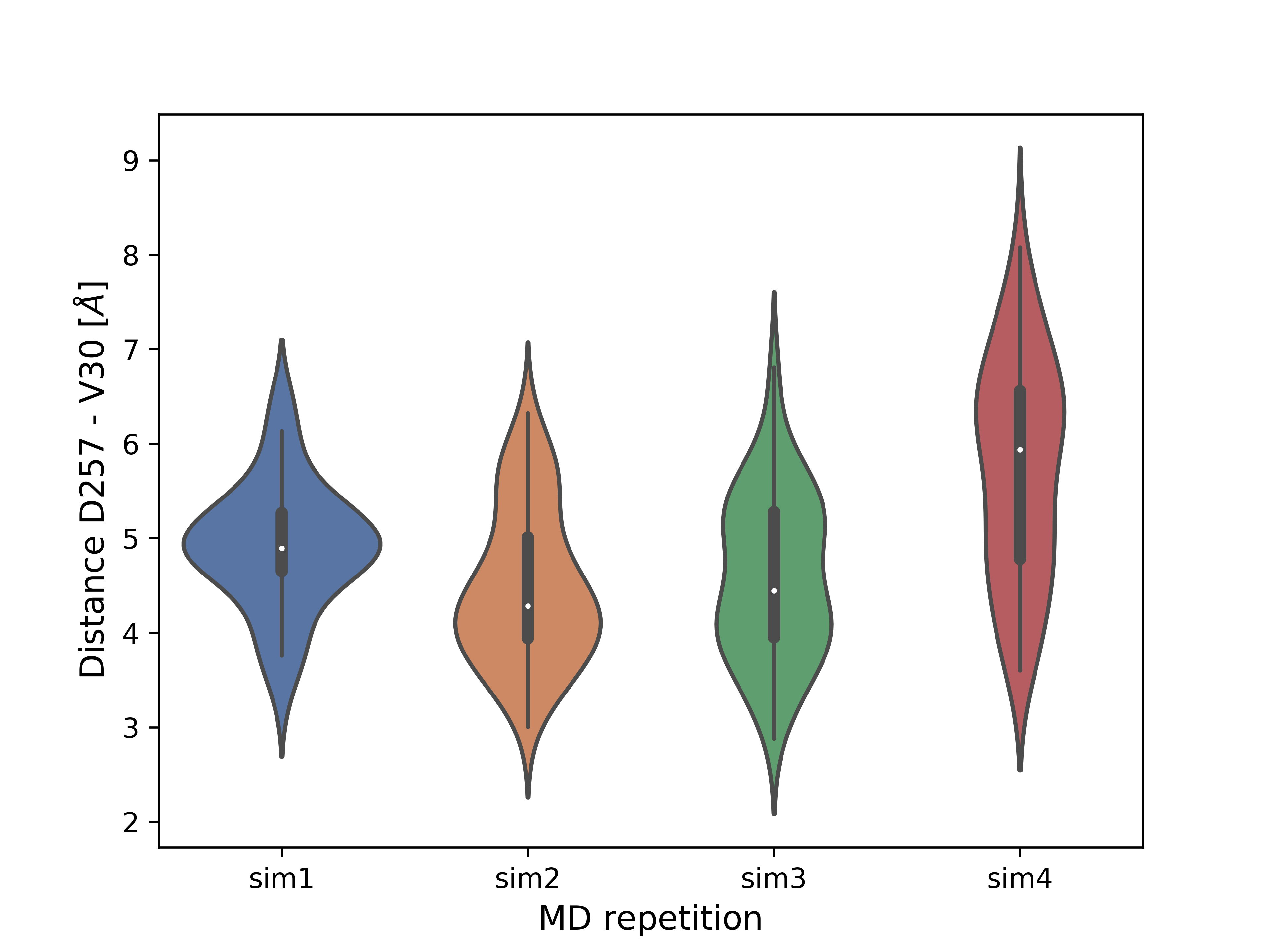 Violin plots for a distance D257-V30 for four repetions of APP SMD-off simulations.
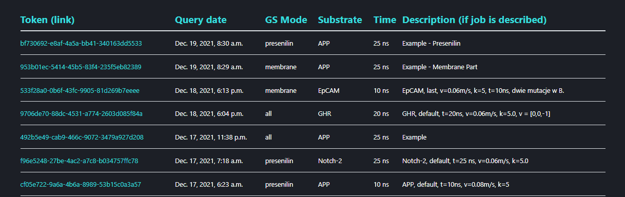
Shared jobs
Clicking the ‘Shared jobs’ leads to a GS-SMD server trajectories data base. The trajectories from MD simulations performed by the users who agreed for their results to be available for public are kept here. In order to submit your results to the ‘Shared jobs list’ on the results page click button.
NGL mouse controls
Left button hold and move to rotate around center
Left button click to pick an atom
Middle button click to center on atom
Middle button hold and move to zoom in and out
Middle button click to center on atom
Right button hold and move to translate in the screen plane
Shift + middle button scroll to adjust clipping
Shift + left button hold and move to zoom in and out
Ctrl + left button hold and move to translate in the screen plane
Ctrl + right button hold and move to rotate in the screen plane